Data Modeling Techniques For Data Warehousing

Data modeling is a process of creating a conceptual representation of the data and its relationships within an organization or system. Dimensional modeling is an advanced technique that attempts to present data in a way that is intuitive and understandable for any user. It also allows for high-performance access, flexibility, and scalability to accommodate changes in business needs.

In this article, I will provide an in-depth overview of data modeling, with a specific focus on Kimball’s methodology. Additionally, I will introduce other techniques used to present data in a user-friendly and intuitive manner. One particularly interesting technique for modern data warehouses is storing data in one wide table, although this approach may not be suitable for all query engines. I will present techniques that can be used in Data Warehouses, Data Lakes, Data Lakehouses, etc. However, it is important to choose the appropriate methodology for your specific use case and query engine.

What is dimensional modeling?

Every dimensional model consists of one or more tables with a multipart key, referred to as the fact table, along with a set of tables known as dimension tables. Each dimension table has a primary key that precisely corresponds to one of the components of the multipart key in the fact table. This distinct structure is commonly referred to as a star schema. In some cases, a more intricate structure called a snowflake schema can be used, where dimension tables are connected to smaller dimension tables

Benefits of dimensional modeling:

Dimensional modeling provides a practical and efficient approach to organizing and analyzing data, resulting in the following benefits:

• Simplicity and understandability for business users.
• Improved query performance for faster data retrieval.
• Flexibility and scalability to adapt to changing business needs.
• Ensured data consistency and integration across multiple sources.
• Enhanced user adoption and self-service analytics.

Now that we have discussed what dimensional modeling is and the value it brings to organizations, let’s explore how to effectively leverage it.

Data and dimensional modeling methodologies

While I intend to primarily focus on Kimball’s methodology, let’s briefly touch upon a few other popular techniques before diving into it.

Inmon methodology

Inmon suggests utilizing a normalized data model within the data warehouse. This methodology supports the creation of data marts. These data marts are smaller, specialized subsets of the data warehouse that cater to specific business areas or user groups. These are designed to provide a more tailored and efficient data access experience for particular business functions or departments.

Data vault

Data Vault is a modeling methodology that focuses on scalability, flexibility, and traceability. It consists of three core components: the Hub, the Link, and the Satellite.

Hubs

Hubs are collections of all distinct entities. For example, an account hub would include account, account_ID, load_date, and src_name. This allows us to track where the record originally came from when it was loaded, and if we need a surrogate key generated from the business key.

Links

Links establish relationships between hubs and capture the associations between different entities. They contain the foreign keys of the related hubs, enabling the creation of many-to-many relationships.

Satellites

Satellites store the descriptive information about the hubs, providing additional context and attributes. They include historical data, audit information, and other relevant attributes associated with a specific point in time.

Data Vault’s design allows for a flexible and scalable data warehouse architecture. It promotes data traceability, auditability, and historical tracking. This makes it suitable for scenarios where data integration and agility are critical, such as in highly regulated industries or rapidly changing business environments.

One big table (OBT) or one wide table

OBT stores data in one wide table. Using one big table, or a denormalized table, can simplify queries, improve performance, and streamline data analysis. It eliminates the need for complex joins, eases data integration, and can be beneficial in certain scenarios. However, it may lead to redundancy, data integrity challenges, and increased maintenance complexity. Consider the specific requirements before opting for a single large table.

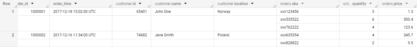
WITH transactions AS (
  SELECT 1000001 AS order_id, TIMESTAMP('2017-12-18 15:02:00') AS order_time,
          STRUCT(65401 AS id, 'John Doe' AS name, 'Norway' AS location) AS customer,
          [
            STRUCT('xxx123456' AS sku, 3 AS quantity, 1.3 AS price),
            STRUCT('xxx535522' AS sku, 6 AS quantity, 500.4 AS price),
            STRUCT('xxx762222' AS sku, 4 AS quantity, 123.6 AS price)
          ] AS orders
  UNION ALL
  SELECT 1000002, TIMESTAMP('2017-12-16 11:34:00'),
        STRUCT(74682, 'Jane Smith', 'Poland') AS customer,
        [
            STRUCT('xxx635354',   4,      345.7),
            STRUCT('xxx828822', 2,      9.5)
        ] AS orders
)


select *


from
transactions

In the case of one wide table we don’t need to join tables. We can use only one table to aggregate data and make analyzes. This method improves performance in BigQuery.

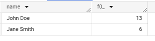
select customer.name, sum(a.quantity)


from
transactions t, UNNEST(t.orders) as a
group by  customer.name

Kimball methodology

The Kimball methodology places significant emphasis on the creation of a centralized data repository known as the data warehouse. This data warehouse serves as a singular source of truth, integrating and storing data from various operational systems in a consistent and structured manner.

This approach offers a comprehensive set of guidelines and best practices for designing, developing, and implementing data warehouse systems. It places a strong emphasis on creating dimensional data models and prioritizes simplicity, flexibility, and ease of use. Now, let’s delve into the key principles and components of the Kimball methodology.

Entity model to dimensional model

In our data warehouses, the sources of data are often found in entity models that are normalized into multiple tables, which contain the business logic for applications. In such a scenario, it can be challenging as one needs to understand the dependencies between tables and the underlying business logic. Creating an analytical report or generating statistics often requires joining multiple tables.

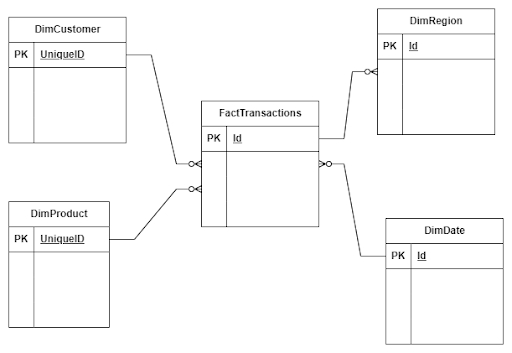
To create a dimensional model, the data needs to undergo an Extract, Transform, and Load (ETL) process to denormalize it into a star schema or snowflake schema. The key activity in this process involves identifying the fact and dimension tables and defining the granularity. The granularity determines the level of detail stored in the fact table. For example, transactions can be aggregated per hour or day.

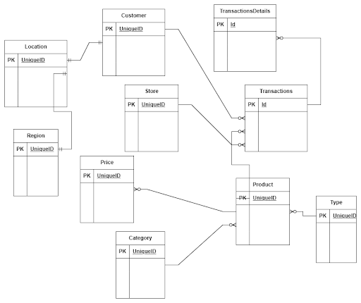
Let’s assume we have a company that sells bikes and bike accessories. In this case, we have information about:

• Transactions
• Stores
• Clients
• Products

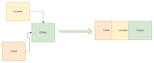
Based on our business knowledge, we know that we need to collect information about sales volume, quantity over time, and segmented by regions, customers, and products. With this information, we can design our data model. The transactions’ table will serve as our fact table, and the stores, clients, and products tables will act as dimensional tables.

Fact table 

A fact table typically represents a business event or transaction and includes the metrics or measures associated with that event. These metrics can encompass various data points such as sales amounts, quantities sold, customer interactions, website clicks, or any other measurable data that offers insights into business performance. The fact table also includes foreign key columns that establish relationships with dimension tables.

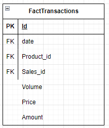
The best practice in the fact table design is to put all foreign keys on the top of the table and then measure.

Fact Tables Types

1. Transaction Fact Tables gives a grain at its lowest level as one row represents a record from the transaction system. Data is refreshed on a daily basis or in real time.
2. Periodic Snapshot Fact Tables capture a snapshot of a fact table at a point in time, like for instance the end of month.
3. Accumulating Snapshot Fact Table summarizes the measurement events occurring at predictable steps between the beginning and the end of a process.
4. Factless Fact Table keeps information about events occurring without any masseurs or metrics. 

Dimension table

A dimension table is a type of table in dimensional modeling that contains descriptive attributes like for instance information about products, its category, and type. Dimension tables provide the context and perspective to the quantitative data stored in the fact table.  

Dimension tables contain a unique key that identifies each record in the table, named surrogate key. The table can contain a business key that is a key from a source system. A good practice is to generate a surrogate key instead of using a business key. 

There are several approaches to creating a surrogate key:

• -Hashing: a surrogate key can be generated using a hash function like MD5, SHA256(e.g. md5(key_1, key_2, key_3) ).
• -Incrementing: a surrogate key that is generated by using a number that is always incrementing (e.g. row_number(), identity).
• -Concatenating: a surrogate key that is generated by concatenating the unique key columns (e.g. concat(key_1, key_2, key_3) ).
• -Unique generated: a surrogate key that is generated by using a function that generates a unique identifier (e.g. GENERATE_UUID())

The method that you will choose depends on the engine that you use to process and store data. It can impact performance of querying data.

Dimensional tables often contain hierarchies.

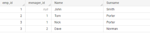
a) For example, the parent-child hierarchy can be used to represent the relationship between an employee and their manager.

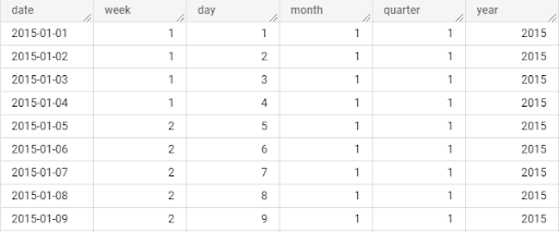
b) Hierarchical relationships between attributes. For example, a time dimension might have attributes like year, quarter, month, and day, forming a hierarchical structure.

Types of dimension tables

Conformed Dimension:

A conformed dimension is a dimension that can be used by multiple fact tables. For example, a region table can be utilized by different fact tables.

Degenerate Dimension:

A degenerate dimension occurs when an attribute is stored in the fact table instead of a dimension table. For instance, the transaction number can be found in a fact table.

Junk Dimension:

This one contains non-meaningful attributes that do not fit well in existing dimension tables, or are combinations of flags and binary values representing various combinations of states.

Role-Playing Dimension:

The same dimension key includes more than one foreign key in the fact table. For example, a date dimension can refer to different dates in a fact table, such as creation date, order date, and delivery date.

Static Dimension:

A static dimension is a dimension that typically never changes. It can be loaded from reference data without requiring updates. An example could be a list of branches in a company.

Bridge Table:

Bridge tables are used when there are one-to-many relationships between a fact table and a dimension table.

Slowly changing dimension

A Slowly Changing Dimension (SCD) is a concept in dimensional modeling. It handles changes to dimension attributes over time in dimension tables. SCD provides a mechanism for maintaining historical and current data within a dimension table as business entities evolve and their attributes change. There are six types of SCD, but the three most popular ones are:

• SCD Type 0: In this type, only new records are imported into dimension tables without any updates.
• SCD Type 1: In this type, new records are imported into dimension tables, and existing records are updated.
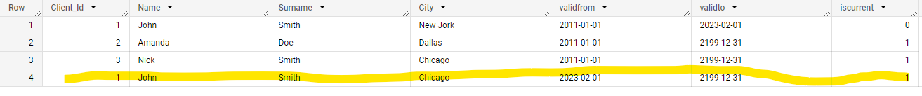
• SCD Type 2: In this type, new records are imported, and new records with new values are created for changed attributes.

For example, when John Smith moves to another city, we use SCD Type 2 to keep information about transactions related to London. In this case, we create a new record and update the previous one. As a result, historical reports will retain information that his purchases were made in London.

MERGE INTO client AS tgt
USING (
    SELECT 
Client_id,
Name,       
Surname,
City
      GETDATE() AS ValidFrom
	‘20199-01-01’ AS ValidTo
from client_stg
) AS src
ON (tgt.Clinet_id = src.Clinet_id AND tgt.iscurrent = 1)
WHEN MATCHED THEN
    UPDATE SET tgt.iscurrent = 0, ValidTo = GETDATE()
WHEN NOT MATCHED THEN
    INSERT (Client_id, name, Surname, City, ValidFrom, ValidTo, iscurrent)
    VALUES (Client_id, name, Surname, City, ValidFrom, ValidTo,1);

This is how SCD 3 looks when we keep new and previous values in separate columns.

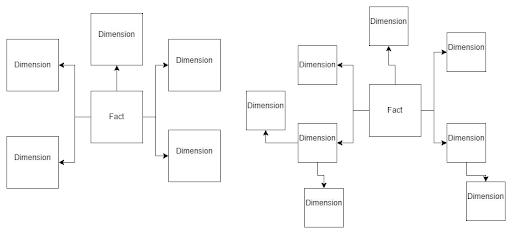
Star schema vs. snowflake schema

The most popular approach to designing a data warehouse is to utilize either a star schema or a snowflake schema. The star schema has fact tables and dimensional tables that are in relation to the fact table. In a star schema, there are fact tables and dimensional tables that are directly related to the fact table. On the other hand, a snowflake schema consists of a fact table, dimension tables related to the fact table, and additional dimensions related to those dimension tables.

The main differences between these two designs lie in their normalization approach. The star schema keeps data denormalized, while the snowflake schema ensures normalization. The star schema is designed for better query performance. The snowflake schema is specifically tailored to handle updates on large dimensions. If you encounter challenges with updates to extensive dimension tables, consider transitioning to a snowflake schema.

Data loading strategies

In our data warehouse, data lake, and data lake house we can have various load strategies like:

Full Load: The full load strategy involves loading all data from source systems into the data warehouse. This strategy is typically used in the case of performance issues or lack of columns that could inform about row modification.

Incremental Load: The incremental load strategy involves loading only new data since the last data load. If rows in the source system can’t be changed, we can load only new records based on a unique identifier or creation date. We need to define a “watermark” that we will use to select new rows.

Delta Load: The delta load strategy focuses on loading only the changed or delta records since the last load. It differs from incremental load in that it specifically targets the delta changes rather than all new records. Delta load strategies can be efficient when dealing with high volumes of data changes and significantly reduce the processing time and resources required.

The most common strategy to load data is to populate dimension tables and then fact tables. The order here is important because we need to use primary keys from dimension tables in fact tables to create relationships between tables. There is an exception. When we need to load a fact table before a dimension table, this technique name is late arriving dimensions.

In this technique, we can create surrogate keys in a dimension table, and update it by ETL process after populating the fact table.